
Pose Graph Optimization (PGO) is the core of the SLAM back-end. Instead of tracking every single landmark or pixel in the environment (which becomes computationally intractable), PGO abstracts the SLAM problem into a graph of robot poses. By treating the poses as variables and the sensor measurements as constraints between them, PGO uses non-linear least-squares optimization to "snap" the trajectory into a globally consistent state, effectively eliminating accumulated drift.
Graph Structure
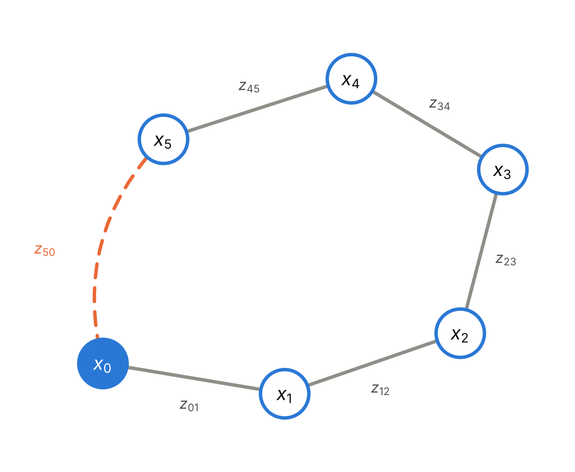
In PGO, the trajectory and measurements are represented as a directed graph.
- Nodes (Vertices): Each node x_i represents the robot's state (pose) at a specific time step i. In 3D space (SE(3)), a node is defined by a 3D translation and a 3D rotation.
- Edges (Constraints): An edge z_ij connects node i to node j and represents a relative measurement (transformation) between those two poses, acting like a mathematical spring.
There are two primary types of edges that make the graph work:
1. Odometry Edges: These connect sequential nodes (e.g., x_{t} and x_{t+1}). They are generated by wheel encoders, visual odometry, or IMU preintegration. They build the initial, drifting trajectory.
2. Loop Closure Edges: These connect non-sequential nodes (e.g., x_{t} and x_{t-100}). They are generated when the front-end recognizes that the robot has returned to a previously visited location. These edges are the key to PGO, as they provide the geometric constraints necessary to correct the drift that accumulated along the odometry edges.
We sum the squared errors of all edges in the entire graph, weighted by their Information matrices (Ω_{ij} = Σ_{ij}^{-1}):
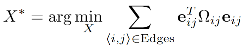
This is a Non-Linear Least Squares optimization problem.
- If an ICP match had high uncertainty (e.g. in a flat hallway), its Information matrix Ω is small, so the "spring" is loose. The optimizer will easily bend it to satisfy other constraints.
- If a loop closure is highly certain, its Ω is large, making the "spring" stiff. The optimizer will force the trajectory to snap to it, propagating corrections backward through the entire history of poses.
Solving the Optimization Problem
Because the poses involve rotations, the error function e_{ij} is non-linear. Therefore, we cannot solve for x^* directly. Instead, we must use iterative solvers.
We linearize the error function around the current state estimate x using a first-order Taylor expansion:

Iterative Solvers
By substituting the linearized error back into the objective function and setting the derivative to zero, we yield a linear system of the form:
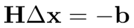
Where H = (J^T)ΩJ, and b = (J^T)Ωe.
Standard algorithms to solve this system include:
- Gauss-Newton: Solves HΔx = -b directly. It is fast but can become unstable if the initial guess is poor.
- Levenberg-Marquardt: Adds a damping factor λ((H + λI)Δx = -b. LM acts like gradient descent when far from the minimum (high λ) and like Gauss-Newton when close (low λ), making it much more robust.
The solver computes the update step Δx, applies it to the state (x ← x ⊕ Δx), and repeats until convergence.
Summary
- Role in SLAM: Pose Graph Optimization (PGO) functions as the back-end of the SLAM architecture. It is responsible for eliminating accumulated sensor drift by optimizing a graph of robot trajectories rather than tracking individual features.
- Graph Formulation: The optimization graph consists of nodes, which represent the robot's pose in SE(3) space at specific time steps, and edges, which represent relative measurements acting as constraints. The two primary edges are sequential odometry edges (which build the trajectory) and non-sequential loop closure edges (which provide the geometry to correct drift).
- Mathematical Objective: PGO is framed as a Non-Linear Least Squares optimization problem. It minimizes the total squared error between predicted and measured edge transformations. These errors are weighted by Information matrices, functioning like "springs" where highly certain measurements pull the trajectory into alignment.
- Optimization Algorithms: Because the constraints involve 3D rotations, the error functions are non-linear and cannot be solved directly. Iterative solvers—such as Gauss-Newton and the more robust Levenberg-Marquardt—linearize the error function to calculate an update step (Δx). This step is continually applied to the state manifold until the system converges on a globally consistent trajectory.